Using R to create complex regression tables for Word and R Markdown

Last updated on Fri, 5. Feb , 2021 11 min read

Overview

This post describes how R can be used to create regression tables that combine multiple models or steps (e.g., stepwise regressions, hierarchical regressions) for several dependent (or outcome) variables. The approach presented here can be used to create tables within R Markdown documents or to create html tables that can be pasted into Word documents.

Background

In 2018, my co-author and I (Brügger and Höchli, 2019) wrote an article in which we examined possible interaction effects between people’s attitude towards the environment and two experimental conditions (dummy variable: recalling environmentally friendly vs. unfriendly behaviour) on many dependent variables.

Using a regression approach to examine whether the predictors interacted, we followed the typical two-step procedure (Cohen, Cohen, West, and Aiken, 2003):

Fit a model with the two predictors that are expected to interact (direct effects)
Fit a second model that also includes the interaction terms of the predictors (interaction effect)

If adding the interaction terms results in a statistically significant improvement of the model, the next step is to do follow-up analyses to visualize and better understand the interaction (Cohen, Cohen, West, and Aiken, 2003; Spiller, Fitzsimons, Lynch, and McClelland, 2013).

Although there are already easy-to-use packages to create nice tables for multiple regression models (or blocks; e.g., apaTables), I could not find an existing solution to create a table that includes the results for several dependent variables. Of course, one could create individual tables for the different dependent variables in R and then combine them into a single table in Word. However, this kind of manual work is both error-prone and cannot be programmatically replicated as it happens outside the R environment.

Benefits, overview, and preview

We looked for a solution to create complex tables programmatically. This has several important benefits:

You can avoid mistakes that occur when copying and adapting R code (e.g., for other dependent variables).
You can avoid mistakes that occur when transferring numbers from R to text editors (e.g., Word) or tables.
In case you need to change something in your analyses (e.g., because a peer-reviewer asks you to use factor scores instead of means to represent your constructs or because you need to include control variables or exclude participants with certain characteristics), you can save a lot of time.
You can quickly adapt the code to conduct similar analyses with other variables (as was the case in this project, in which we examined similar processes in the context of health).
The analyses can be shared and replicated quickly and effortlessly.
The code can directly be included in R Markdown documents (to create papers directly from R).
The table can be adapted to suit different requirements; for example, you can include other statistical information.

The approach presented here includes the following five steps:

Preparation (get the data ready)
Fit additive regression models (direct effects) and save the relevant statistics
Fit multiplicative regression models (direct and interactive effects) and save the relevant statistics
Compare the models
Create the table

The results will look more or less like this:

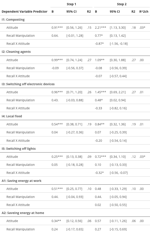
Figure 1. Regression table with additive and interaction effects for multiple dependent variables.

1. Preparation

Check if the necessary packages are available and install them if they are not:

if (!require("pacman")) install.packages("pacman")
pacman::p_load(
"tidyverse", # data handling & cleaning
"purrr", # applying the linear regression function to several dependent variables
"sjlabelled", # working with item labels (e.g., display their actual content)
"kableExtra", # for customizing and displaying tables
"broom", # for extracting information from linear models
"gtools") # to convert p-values into significance stars

To be able to replicate the code and create the table, you can either manually download the file “df_study1.RData” from https://osf.io/mbgxh, put it in the folder where your R code is located (or set the working directory accordingly), and load the data into R:

load("df_study1.RData") # this only works if data is downloaded manually

Or you can access the data directly from R:

library("httr")
url <- 'https://osf.io/62ya5//?action=download'
filename <- 'df_study1.RData'
GET(url, write_disk(filename, overwrite = TRUE))
load("df_study1.RData")

The data includes a lot of variables and two experimental conditions that are not needed for this analysis. Reduce the data to the relevant variables and cases (for a better overview):

# define dependent variables, see also https://www.adrianbruegger.com/post/variable-selection-with-lists/
dep_vars_env <- c("env_int1","env_int2","env_int3","env_int4","env_int5","env_app1","env_app2","env_app3")

# keep only the necessary variables
df <- df %>%
select("condition", "env_att_scale", # predictors (experimental condition and environmental attitude)
all_of(dep_vars_env)) # dependent variables


# remove experimental conditions that are not required for this analysis (conditions 3 and 4 concerned health rather than the environment)
df <- filter(df, condition < 3)


# The results are easier to interpret if negative condition is the reference category
df$condition <- as.numeric(recode(df$condition, "2" = "0", "1" = "1"))

2. Fit the additive models

Fit an additive model for each dependent variable (Step 1) and extract the relevant statistical information:

# Use “map” from the package purrr to fit a linear regression model for each dependent variable:
env_additive_models <- df %>%
dplyr::select(one_of(dep_vars_env)) %>% # select dependent variables
map(~lm(.x ~ env_att_scale + condition, data = df)) # use "map" to conduct the defined linear model with each dependent variable (.x)


#For each dependent variable, extract statistical information for both predictors (B, SE, t, p, CI)
env_additive_model_CI <- env_additive_models %>%
# extract relevant statistics from each model (ie for each dv)
map_df(broom::tidy, conf.int=TRUE) %>%
# remove the intercepts (not needed for the target journal)
filter(term !="(Intercept)") %>%
# add stars to denote level of significance
mutate(stars = gtools::stars.pval(p.value)) %>%
# get names of models (dvs)
mutate(dependent = rep(names(env_additive_models),each=2)) %>%
# get item content (this only works with dataframes that do include the item contents as attributes, e.g., by using the package qualtRics)
mutate(wording = lmap(env_additive_models, function(x) rep(map(.x=x, .f=function(x) attributes(x$residuals)$label),each=2)))

To be able to properly combine the information of the additive models with the interaction models at a later stage, it is necessary that the information from the additive model has the same number of rows as the (longer) interaction table and that the relevant information is located in the correct rows. To achieve this, empty cells need to be added where later the interaction terms will be placed (thanks to: https://stackoverflow.com/questions/46814145/baser-how-to-add-empty-row-after-x-number-of-rows). Moreover, the stats need to be saved as numeric variables to be able to compute R2-change later.

# add an empty row after two rows to make table same length as interaction model (otherwise they cannot be merged properly)
# How many rows need to be added?
N <- 1
# After how many rows with actual content?
after_rows <- 2
env_additive_model_CI <- do.call(rbind, lapply(split(env_additive_model_CI, ceiling(1:NROW(env_additive_model_CI)/after_rows)),
function(a) rbind(a, replace(a[1:N,], TRUE, ""))))
# ensure that relevant columns are numeric
env_additive_model_CI <- env_additive_model_CI %>%
mutate_at(vars(estimate, std.error, statistic, p.value, conf.low, conf.high),list(~as.numeric(.)))
# TODO remove if above new line works
# mutate_at(vars(estimate, std.error, statistic, p.value, conf.low, conf.high),funs(as.numeric)) # this is now deprecated

Get and save the statistical information for the overall model, adjust the length of the object in which the stats are saved, make again sure that all stats columns are numeric, and combine the statistical information regarding the predictors and the overall model:

# get model stats (R2, p, etc.) for each model and dv
env_additive_model_stats <- df %>%
dplyr::select(one_of(dep_vars_env)) %>%
map(~lm(.x ~ env_att_scale + condition, data = df)) %>%
map(summary) %>%
map_df(broom::glance) %>%
mutate(stars = gtools::stars.pval(p.value)) %>%
setNames(paste0("m_", names(.)))

# add empty row after two rows to make sure object has same length as other parts of the final table (ie step 2 with more predictors)
after_rows <- 1
N <- 2
env_additive_model_stats <- do.call(rbind, lapply(split(env_additive_model_stats, ceiling(1:NROW(env_additive_model_stats)/after_rows)),
function(a) rbind(a, replace(a[1:N,], TRUE, ""))))

# make sure relevant variables are numeric
env_additive_model_stats <- env_additive_model_stats %>% mutate_at(vars(m_r.squared, m_adj.r.squared, m_sigma, m_statistic, m_p.value, m_df),funs(as.numeric))

# combine stats for predictors and models
env_additive_all <- cbind(env_additive_model_CI,env_additive_model_stats)
# rename columns so they have a unique name (otherwise merging will not work later)
colnames(env_additive_all) <- paste0("st1_",colnames(env_additive_all))

3. Fit the interaction models

The procedure for the interaction models is almost exactly the same. The only difference is that no extra rows need to be added:

#Fit interaction model (Step 2)
env_interaction_models <- df %>%
dplyr::select(one_of(dep_vars_env)) %>% #
map(~lm(.x ~ env_att_scale * condition, data = df))
# get stats and confidence intervals for each model and dv
env_interaction_model_CI <- env_interaction_models %>%
map_df(broom::tidy, conf.int=TRUE) %>%
filter(term !="(Intercept)") %>%
rename(predictor = term) %>%
mutate(stars = gtools::stars.pval(p.value))
# get model stats for each model and each dev
env_interaction_model_stats <- df %>%
dplyr::select(one_of(dep_vars_env)) %>% #
map(~lm(.x ~ env_att_scale * condition, data = df)) %>%
map(summary) %>%
map_df(broom::glance) %>%
mutate(stars = gtools::stars.pval(p.value)) %>%
setNames(paste0("m_", names(.)))
# add empty row after two rows to make sure that different "tables" can be merged without problems
after_rows <- 1
N <- 2
env_interaction_model_stats <- do.call(rbind, lapply(split(env_interaction_model_stats, ceiling(1:NROW(env_interaction_model_stats)/after_rows)),
function(a) rbind(a, replace(a[1:N,], TRUE, ""))))
# make sure all relevant variables are numeric
env_interaction_model_stats <- env_interaction_model_stats %>% mutate_at(vars(m_r.squared, m_adj.r.squared, m_sigma, m_statistic, m_p.value, m_df),funs(as.numeric))
# merge "tables" with stats concerning predictors and full model
env_interaction_all <- cbind(env_interaction_model_CI,env_interaction_model_stats)
# rename columns so they have a unique name (for joining without problems)
colnames(env_interaction_all) <- paste0("st2_",colnames(env_interaction_all))

4. Compare the additive and interaction models

Use F tests to compare the additive and interaction model for each dependent variable and prepare the statistical information so it can be combined into a single table together with the statistical information of the additive and interaction models:

model_comparisions <- map2_df(env_additive_models, env_interaction_models, stats::anova) %>%
dplyr::select(F, "Pr(>F)")# only keep necessary columns
# delete uneven rows (they don't contain any information for the two relevant columns)
model_comparisions <- model_comparisions[c(FALSE,TRUE),]
# add stars to indicate level of significane
model_comparisions$stars_m <- gtools::stars.pval(model_comparisions$"Pr(>F)")
# add empty columns to get object with same length
after_rows <- 1
N <- 2
model_comparisions <- do.call(rbind, lapply(split(model_comparisions, ceiling(1:NROW(model_comparisions)/after_rows)),
function(a) rbind(a, replace(a[1:N,], TRUE, ""))))
# combine relevant tables / dataframes
env_attitude_models <- cbind(env_additive_all,env_interaction_all)
env_attitude_models <- as.tibble(cbind(env_attitude_models,model_comparisions))

One thing that is missing is the extent to which R2 changes when the interaction terms are added (i.e., R2 difference between Step 1 and Step 2; last column in the table). Moreover, some formatting is required (e.g., rounding numbers, adding brackets around the confidence intervals).

table_env_attitudes <- env_attitude_models %>%
mutate(r2_ch = as.numeric(st2_m_r.squared)-as.numeric(st1_m_r.squared)) %>%
# rounding for all variables at once does not work properly:
# mutate_if(is.numeric, round, 2) %>%
# manually round to two digits
mutate(st1_estimate = sprintf("%0.2f",round(st1_estimate,2))) %>%
mutate(st1_conf.low = sprintf("%0.2f",round(st1_conf.low,2))) %>%
mutate(st1_conf.high = sprintf("%0.2f",round(st1_conf.high,2))) %>%
mutate(st1_m_r.squared = sprintf("%0.2f",round(st1_m_r.squared,2))) %>%
mutate(st2_estimate = sprintf("%0.2f",round(st2_estimate,2))) %>%
mutate(st2_conf.low = sprintf("%0.2f",round(st2_conf.low,2))) %>%
mutate(st2_conf.high = sprintf("%0.2f",round(st2_conf.high,2))) %>%
mutate(st2_m_r.squared = sprintf("%0.2f",round(st2_m_r.squared,2))) %>%
mutate(r2_ch = sprintf("%0.2f",round(r2_ch,2))) %>%

# get rid of NAs in last r2_change column
mutate(r2_ch = replace_na(r2_ch, "")) %>%
mutate(r2_ch = str_remove(r2_ch, "NA")) %>%
# add stars to Bs
unite(st1_estimate, c("st1_estimate","st1_stars"), sep = "") %>%
unite(st2_estimate, c("st2_estimate","st2_stars"), sep = "") %>%
unite(r2_ch, c("r2_ch","stars_m"), sep = "") %>%
# re-order columns
dplyr::select(st1_dependent,st1_wording,st2_predictor, st1_estimate, st1_conf.low, st1_conf.high,st1_m_r.squared,
st2_estimate, st2_conf.low, st2_conf.high,st2_m_r.squared,r2_ch)
# add new column with better names of predictors
table_env_attitudes$predictors <- rep(c("Attitude","Recall Manipulation","Recall X Attitude"), 8)
# re-order and select relevant columns
table_env_attitudes <- table_env_attitudes %>% dplyr::select(st1_dependent,st1_wording,predictors, everything(),-st2_predictor)

# combine CI upper and lower into one column
table_env_attitudes <- table_env_attitudes %>%
unite(CI_1, c("st1_conf.low","st1_conf.high"), sep = ", ") %>%
unite(CI_2, c("st2_conf.low","st2_conf.high"), sep = ", ")
# add brackets
table_env_attitudes$CI_1 <- paste0("[",table_env_attitudes$CI_1,"]")
table_env_attitudes$CI_2 <- paste0("[",table_env_attitudes$CI_2,"]")
# remove NAs / empty CIs from step 1
# replace 0. with . in R2
table_env_attitudes <- table_env_attitudes %>%
mutate(CI_1 = str_remove(CI_1, "\\[, \\]|\\[NA, NA\\]")) %>%
mutate(st1_estimate = replace_na(st1_estimate, "")) %>%
mutate(st1_m_r.squared = replace_na(st1_m_r.squared, "")) %>%
mutate(st2_m_r.squared = replace_na(st2_m_r.squared, "")) %>%
mutate(st1_estimate = str_remove(st1_estimate, "NA")) %>%
mutate(st1_m_r.squared = str_remove(st1_m_r.squared, "NA")) %>%
mutate(st2_m_r.squared = str_remove(st2_m_r.squared, "NA")) %>%
mutate(st1_m_r.squared = str_replace(st1_m_r.squared, "0.",".")) %>%
mutate(st2_m_r.squared = str_replace(st2_m_r.squared, "0.",".")) %>%
mutate(r2_ch = str_replace(r2_ch, "0.","."))

5. Create the table

I used kableExtra to prepare the final table. The following code will display the table in the R Studio Viewer. The table can be copied and pasted into Word, where you can do some final formatting. Tables can of course also be directly added to R Markdown documents:

table_env_attitudes %>%
# remove name of dependent variable
dplyr::select(-st1_dependent,-st1_wording) %>%
kableExtra::kable(format = "html", digits=2,
col.names = c("Dependent Variable\nPredictor","B","95% CI","R2","B","95% CI","R2","R^2ch"),escape = F) %>%
kableExtra::add_header_above(c(" " = 1, "Step 1" = 3, "Step 2" = 4)) %>%
kableExtra::group_rows("I1: Composting", 1, 3) %>%
kableExtra::group_rows("I2: Cleaning agents", 4, 6) %>%
kableExtra::group_rows("I3: Switching off electronic devices", 7, 9) %>%
kableExtra::group_rows("I4: Local food", 10,12) %>%
kableExtra::group_rows("I5: Switching off lights", 13,15) %>%
kableExtra::group_rows("A1: Saving energy at work", 16,18) %>%
kableExtra::group_rows("A2: Saveing energy at home", 19,21) %>%
kableExtra::group_rows("A3: Reduce CO2", 22,24) %>%
kableExtra::footnote(general = "Environmentally unfriendly behavior were coded as 0, environmentally friendly behavior as 1; *** p < .001, ** p < .01, * p < .05, . < .10.") %>%
kableExtra::kable_styling(bootstrap_options = c("hover"),full_width = F,font_size=12)

References

Brügger, A., & Höchli, B. (2019). The role of attitude strength in behavioral spillover: Attitude matters—but not necessarily as a moderator. Frontiers in Psychology, 10(1018), 1–24. https://doi.org/10.3389/fpsyg.2019.01018

Cohen, J., Cohen, P., West, S. G., & Aiken, L. S. (2003). Applied multiple regression/correlation analysis for the behavioral sciences (3rd ed.). Lawrence Erlbaum.

Spiller, S. A., Fitzsimons, G. J., Lynch, J. G., & McClelland, G. H. (2013). Spotlights, floodlights, and the magic number zero: Simple effects tests in moderated regression. Journal of Marketing Research, 50(2), 277–288. https://doi.org/10.1509/jmr.12.0420