Using R to create variations of images for research projects

Background

In our research group we recently prepared an experiment that is interested in how different carbon labels may affect consumers. More specifically, we wanted to compare the following three labels to a control condition (without carbon label):

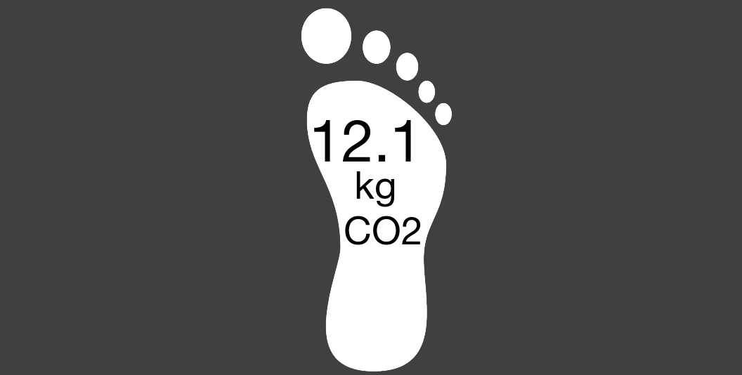
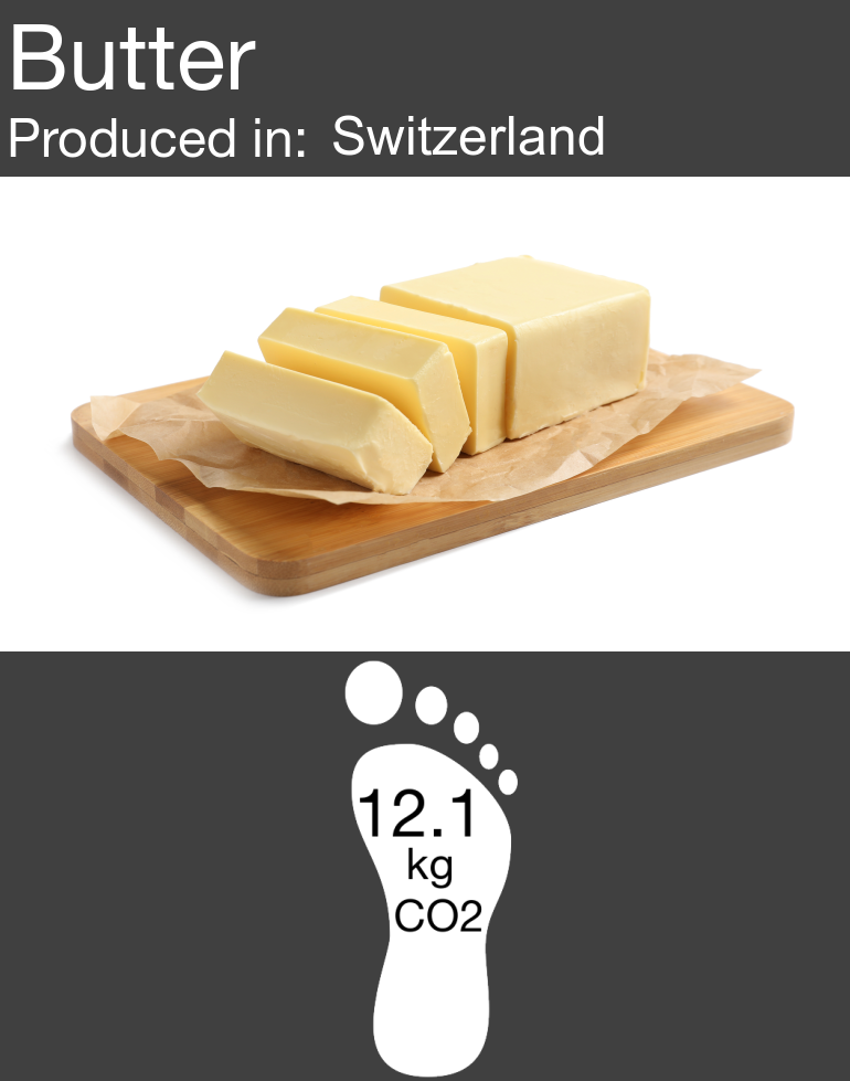
1. The absolute label simply shows the amount of CO2 that is caused by producing a food item
   

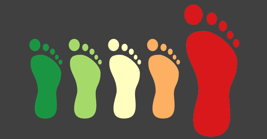
2. The traffic label uses five colours to indicate the climate impact of the product relative to comparable products (similar to the nutri-score label and the energy label)
   

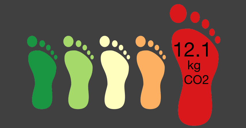
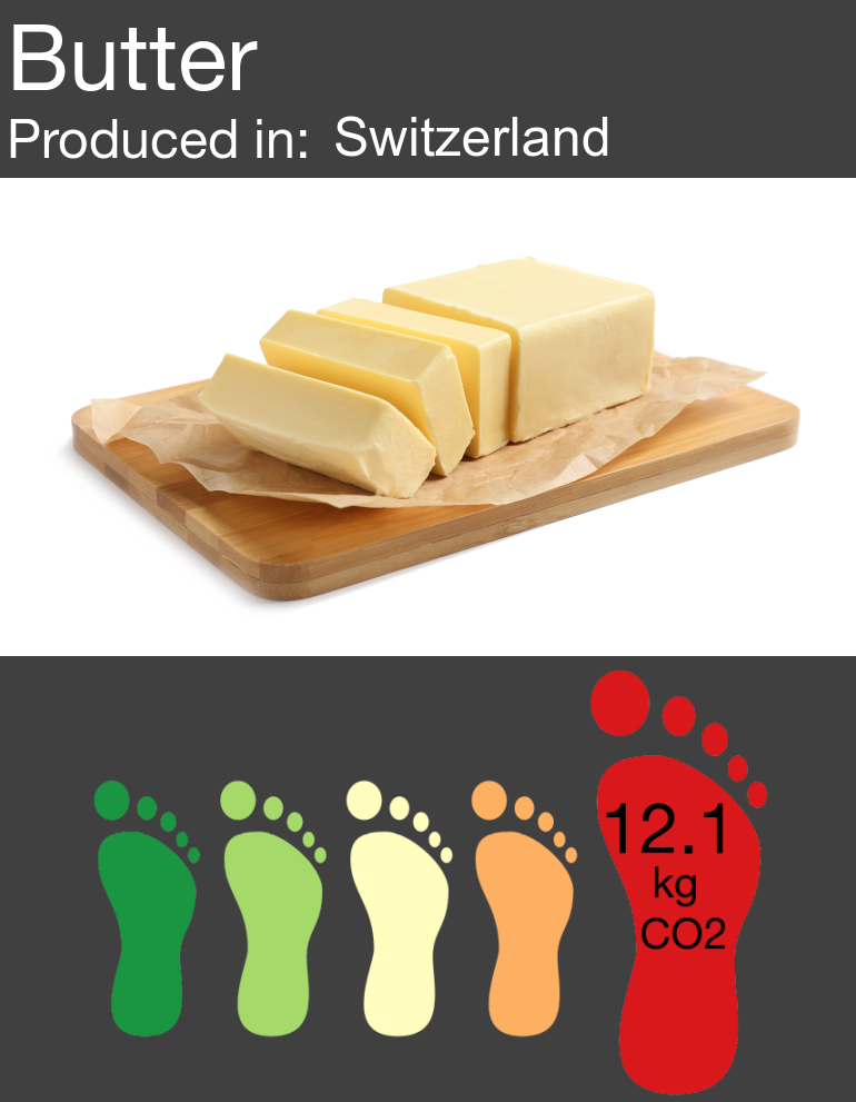
3. The combined label uses both the numeric information from A) and the colours from B)
   

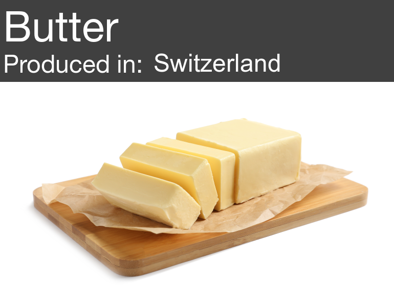
For the experiment, we wanted to use images that include the name of the product, its origin, and the label (or no label in the control condition). The initial approach to create the images was to manually assemble the relevant information in PowerPoint and then save each image. However, with approximately 150 images to create, this turned out to be a very long and error-prone process. Things such as changing the design (e.g., background colour, font type / size) took forever and there was a considerable risk of adding wrong information to the images.

To automate the process and make it easier to quickly apply changes to all images, I turned to R and the image processing package magick. A really nice side effect is that the process of creating the images is now more transparent. Moreover, the code can be relatively easy be adapted for other projects.

Preparation

Before doing anything in R, it is a good idea to prepare all the information so R can access and process it. More specifically, I prepared a table in which each line represents a product and the columns contain relevant information such as the name of the product, where it is produced, the amount of CO2 that is emitted during the production, the name of the image file that shows the product, and the path to the folder that contains the image.

Building elements

Depending on the experimental condition, the images should consist of 1-3 elements with varying content:

1. Header with product name, origin, and product image
2. Label (or no label in the control condition)
3. Text indicating the carbon emissions of the product (in the conditions “absolute” and “combined”)

To combine these elements into a single image with magick, each element or combination of elements needs to be saved as an image. Magick can combine such elements in different ways. If the three elements had consistently the same dimensions (height and width), one could simply create a background / base layer with fixed dimensions and then “paste” the elements where they belong with the r function image_composite. However, the height of the used product images varied and this simple way didn’t work; the three parts cannot be directly put on a base layer (or at least I couldn’t figure out how).

The alternative is to first create the header. Then the other parts are created (traffic label / label with amount of CO2 / combined label) and put below the header.

Details and code

Below you find the code for creating the images. The code, the data, and images are also availabe on my github repository.

Load packages (install if not yet available):

if (!require("pacman")) install.packages("pacman")
pacman::p_load("tidyverse","readxl", "stringr","magick")

Import and prepare data (incl. adjusting the path to the prodcut images):

# import specific sheet from Excel file
df <- readxl::read_excel("../product_info.xlsx", sheet = "stimuli_data")

# indicate path to product images
df$image_path <- stringr::str_c("../images/originals/products/",df$image_product)
  
# update path to label templates
df$label_path <- stringr::str_c("../images/originals/labels/",df$label,"_V2_1.png")

Create the header:

# create head / basic image consisting of product name and image 
# lapply applies the function defined below for all elements / rows in the column "image_path" (could also be a different column with unique information)
img_lst <- lapply(seq_along(df$image_path), function(i){
  # create white background
  background <- image_blank(width = 770, height = 160, color = "grey25")
  # get product name
  product_en <- df$product_en[[i]]
  # get image
  product_image <- image_read(df$image_path[[i]]) 
  # add text to background
  base <- background %>% 
    # add product name from variable "product_en"
    image_annotate(paste0(df$product_en[[i]]), size = 82, color = "white", weight=700, 
                   location = "+6+2", font= "Helvetica") %>% 
    # add fix text for place of production 
    image_annotate("Produced in:", size = 48, color = "white", weight=500, 
                   location = "+6+96", font= "Helvetica") %>% 
    # add origin from variable "origin_en"
    image_annotate(paste0(df$origin_en[[i]]), size = 48, color = "white", weight=500, 
                   location = "+300+96") 
  # create image consisting of base with text + image
  img <- c(base,product_image)
  # explain how to combine these elements
  image_append(image_scale(img, "770"), stack = TRUE) %>% 
    # save image
    image_write(path = paste0("../images/final/", "control_",product_en, ".png"), format = "png") #, quality = 50) #, compression = 
})

The result looks like this and is actually also the control condition:

The next step is to prepare the foot for the experimental condition “absolute” (single foot with amount of CO2).

# very similar logic as above
img_lst <- lapply(seq_along(df$image_path), function(i){
  # get relevant information
  product_en <- df$product_en[[i]]
  image_read("../images/originals/labels/White_V2.png")  %>% 
    # print information about CO2 in correct place
    image_annotate(paste0(sprintf("%.1f",round(df$co2[[i]], 1))), size = 83, color = "black", weight=700, 
                   location = "+73+150",font= "Helvetica") %>% 
    # add constant information kg/CO2
    image_annotate(" kg\nCO2", size = 55, color = "black", weight=700, 
                   location = "+89+230",font= "Helvetica") %>% 
    image_background("grey25") %>% 
    image_border("grey25", "400x0") %>% # add border so that foot will be similarly large as in traffic version
    image_write(path = paste0("../images/absolute/", product_en, ".png"), format = "png") #, quality = 50) #, compression = 
})

# move text for large numbers, otherwise it doesn't appear in the correct place (outside the foot)
# overwrite  products with co2 >=10
df_big <- df %>% filter(co2 >=10)
img_lst <- lapply(seq_along(df_big$image_path), function(i){
  product_en <- df_big$product_en[[i]]
  image_read("../images/originals/labels/White_V2.png")  %>% 
    image_annotate(paste0(sprintf("%.1f",round(df_big$co2[[i]], 1))), size = 83, color = "black", weight=700, 
                   location = "+40+150",font= "Helvetica") %>% 
    image_annotate(" kg\nCO2", size = 55, color = "black", weight=700, 
                   location = "+89+230",font= "Helvetica") %>% 
    image_background("grey25") %>% 
    image_border("grey25", "400x0") %>% # add border so that foot will be similarly large as in traffic version
    image_write(path = paste0("../images/absolute/", product_en, ".png"), format = "png") #, quality = 50) #, compression = 
})

And then add it to the header.

# combine image and foot (all absolute images)
img_lst <- lapply(seq_along(df$image_path), function(i){
  product_en <- df$product_en[[i]]
  header <- image_read(path = paste0("../images/final/control_", df$product_en[[i]], ".png")) 
  label  <- image_read(path = paste0("../images/absolute/", df$product_en[[i]], ".png")) 
  img <- c(header,label)
  image_append(image_scale(img,"770"), stack = TRUE) %>% 
    image_write(path = paste0("../images/final/", "absolute_", product_en, ".png"), format = "png") #, quality = 50) #, compression = 
})

The result looks like this:

Then we create the images for the experimental condition “traffic” (“relative” feet without indication of CO2).

img_lst <- lapply(seq_along(df$product_en), function(i){
  product_en <- df$product_en[[i]]
  image_read(df$label_path[[i]]) %>% 
    image_background("grey25") %>% 
    image_border("grey25", "80x10") %>% # add border so that image will end up smaller in the final version
    image_crop(geometry="1200x445",repage=TRUE) %>% # crop bottom to make picture less high
    image_write(path = paste0("../images/traffic/", product_en, ".png"), format = "png") #, quality = 50) #, compression = 
})

# combine image and foot and save
img_lst <- lapply(seq_along(df$image_path), function(i){
  product_en <- df$product_en[[i]]
  header <- image_read(path = paste0("../images/final/control_", df$product_en[[i]], ".png")) 
  label  <- image_read(path = paste0("../images/traffic/", df$product_en[[i]], ".png")) 
  img <- c(header,label)
  image_append(image_scale(img,"770"), stack = TRUE) %>% 
    image_write(path = paste0("../images/final/", "traffic_", product_en, ".png"), format = "png") #, quality = 50) #, compression = 
})

Resulting example image:

And finally the code for the combined version. Note that these images need to be created separately for each level of the label (A, B, C, D, E) to ensure that the text is placed on the correct position (different for each enlarged foot).

# do A - Labels
df_A <- df %>% filter(label=="A")

img_lst <- lapply(seq_along(df_A$label_path), function(i){
  product_en <- df_A$product_en[[i]]
  image_read(df_A$label_path[[i]]) %>% 
    image_annotate(paste0(sprintf("%.1f",round(df_A$co2[[i]], 1))), size = 70, color = "black", weight=700, 
                   location = "+40+120",font= "Helvetica") %>% 
    image_annotate(" kg\nCO2", size = 43, color = "black", weight=700, 
                   location = "+50+190",font= "Helvetica") %>% 
    image_background("grey25") %>% 
    image_border("grey25", "80x10") %>% # add border so that image will end up smaller in the final version
    image_crop(geometry="1200x435",repage=TRUE) %>% # crop bottom to make picture less high
    image_write(path = paste0("../images/combined/", product_en, ".png"), format = "png") #, quality = 50) #, compression = 
})


# do B - Labels

df_B <- df %>% filter(label=="B")

img_lst <- lapply(seq_along(df_B$label_path), function(i){
  product_en <- df_B$product_en[[i]]
  image_read(df_B$label_path[[i]])  %>% 
    image_annotate(paste0(sprintf("%.1f",round(df_B$co2[[i]], 1))), size = 70, color = "black", weight=700, 
                   location = "+164+120",font= "Helvetica") %>% 
    image_annotate(" kg\nCO2", size = 43, color = "black", weight=700, 
                   location = "+174+190",font= "Helvetica") %>% 
    image_background("grey25") %>% 
    image_border("grey25", "80x10") %>% # add border so that image will end up smaller in the final version
    image_crop(geometry="1200x435",repage=TRUE) %>% # crop bottom to make picture less high
    image_write(path = paste0("../images/combined/", product_en, ".png"), format = "png") #, quality = 50) #, compression = 
})



# C - Labels
df_C <- df %>% filter(label=="C")

img_lst <- lapply(seq_along(df_C$label_path), function(i){
  product_en <- df_C$product_en[[i]]
  image_read(df_C$label_path[[i]])  %>% 
    image_annotate(paste0(sprintf("%.1f",round(df_C$co2[[i]], 1))), size = 70, color = "black", weight=700, 
                   location = "+284+120",font= "Helvetica") %>% 
    image_annotate(" kg\nCO2", size = 43, color = "black", weight=700, 
                   location = "+294+190",font= "Helvetica") %>% 
    image_background("grey25") %>% 
    image_border("grey25", "80x10") %>% # add border so that image will end up smaller in the final version
    image_crop(geometry="1200x435",repage=TRUE) %>% # crop bottom to make picture less high
    image_write(path = paste0("../images/combined/", product_en, ".png"), format = "png") #, quality = 50) #, compression = 
})


# D - Labels

df_D <- df %>% filter(label=="D")

img_lst <- lapply(seq_along(df_D$label_path), function(i){
  product_en <- df_D$product_en[[i]]
  image_read(df_D$label_path[[i]])  %>% 
    image_annotate(paste0(sprintf("%.1f",round(df_D$co2[[i]], 1))), size = 70, color = "black", weight=700, 
                   location = "+424+120",font= "Helvetica") %>% 
    image_annotate(" kg\nCO2", size = 43, color = "black", weight=700, 
                   location = "+433+190",font= "Helvetica") %>% 
    image_background("grey25") %>% 
    image_border("grey25", "80x10") %>% # add border so that image will end up smaller in the final version
    image_crop(geometry="1200x440",repage=TRUE) %>% # crop bottom to make picture less high
    image_write(path = paste0("../images/combined/", product_en, ".png"), format = "png") #, quality = 50) #, compression = 
})


# E - Labels
df_E <- df %>% filter(label=="E")

img_lst <- lapply(seq_along(df_E$label_path), function(i){
  product_en <- df_E$product_en[[i]]
  image_read(df_E$label_path[[i]])  %>% 
    image_annotate(paste0(sprintf("%.1f",round(df_E$co2[[i]], 1))), size = 70, color = "black", weight=700, 
                   location = "+549+120",font= "Helvetica") %>% 
    image_annotate(" kg\nCO2", size = 43, color = "black", weight=700, 
                   location = "+559+190",font= "Helvetica") %>% 
    image_background("grey25") %>% 
    image_border("grey25", "80x10") %>% # add border so that image will end up smaller in the final version
    image_crop(geometry="1200x445",repage=TRUE) %>% # crop bottom to make picture less high
    image_write(path = paste0("../images/combined/", product_en, ".png"), format = "png") #, quality = 50) #, compression = 
})

# overwrite  products with co2 >=10 so that text appears in good place
df_E <- df %>% filter(label=="E") %>% filter(co2 >=10)

img_lst <- lapply(seq_along(df_E$label_path), function(i){
  product_en <- df_E$product_en[[i]]
  image_read(df_E$label_path[[i]])  %>% 
    image_annotate(paste0(sprintf("%.1f",round(df_E$co2[[i]], 1))), size = 70, color = "black", weight=700, 
                   location = "+520+120",font= "Helvetica") %>% 
    image_annotate(" kg\nCO2", size = 43, color = "black", weight=700, 
                   location = "+559+190",font= "Helvetica") %>% 
    image_background("grey25") %>% 
    image_border("grey25", "80x10") %>% # add border so that image will end up smaller in the final version
    image_crop(geometry="1200x445",repage=TRUE) %>% # crop bottom to make picture less high
    image_write(path = paste0("../images/combined/", product_en, ".png"), format = "png") #, quality = 50) #, compression = 
})


# combine image and foot (all combined images)
img_lst <- lapply(seq_along(df$image_path), function(i){
  product_en <- df$product_en[[i]]
  header <- image_read(path = paste0("../images/final/control_", df$product_en[[i]], ".png")) 
  label  <- image_read(path = paste0("../images/combined/", df$product_en[[i]], ".png")) 
  img <- c(header,label)
  image_append(image_scale(img,"770"), stack = TRUE) %>% 
    image_write(path = paste0("../images/final/", "combined-", product_en, ".png"), format = "png") #, quality = 50) #, compression = 
})

Resulting example image:

Conclusion

This is the first time I used magick. I was really surprised how powerful the package is and how quickly the code for this quite complex task was written. Now that this code is available, it will be easier still for future me and others with similar tasks on their hand to create such visual stimuli.

Credit

Parts of the crucial lapply function was adapted from https://github.com/ropensci/magick/issues/297.